Long-run frequency over repeated trials.
Ex, repeatedly flipping a coin, shooting electrons at a double slit.
systematic random sampling from a population.
Ex, survey of random voters, random assignment to treatment/control group. Randomness comes from experimenters' actions.
Subjective uncertainty about an outcome.
Ex, chance that Trump is elected, th digit of is . Could be broad intersubjective agreement.
2 Where does Prior Come From?
2.1 Subjective Beliefs
Subjective beliefs bring all relevant information to bear straightforward interpretation of posterior. But posterior is therefore subjective.
2.2 "Objective" or "Vague" Prior
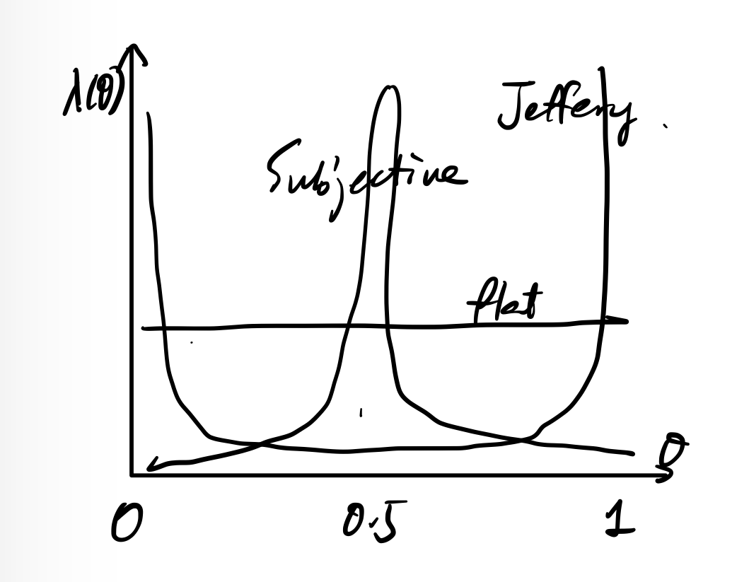
Using default prior removes subjectivity. Like flat prior on .
Example
If is flat prior on , and , then
We also have Jeffrey's prior (recall Fisher information). In this case, recall this formula, we have Then when is small, has higher density when is "changing faster".
Example (Binomial)
If , So as or . And we can see that
Take coin tossing as an example:
2.2.1 Intersubjective Agreement
Data may effectively rule out most values. This will make posterior uncontroversial.
Example
. Observe . The standard deviation so likelihood for outside . So all "reasonable" priors may be close to flat on . So
"Data swamps everyone's prior."
For , recall , and note that , so .
Now apply bias-variance tradeoff:
Examine Jeffrey's prior again: which grows rapidly. This shows prior "expects" to be large.
2.3 Prior or Concurrent Experience
Example
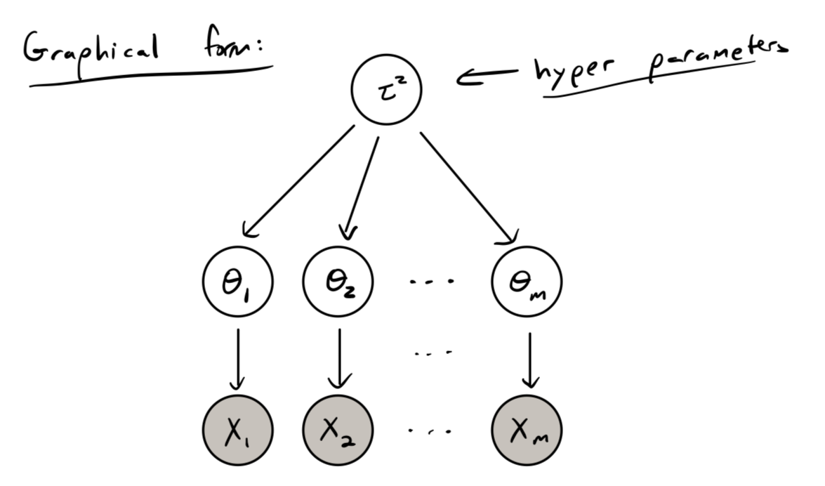
Estimate same-side bias for coin flippers. Flipper has trials, "true" same-side probability . Construct a hierarchical model: for flippers , ,[2], . So and If is large, may be "almost known", so choice of doesn't matter much.
2.3.1 Flexibility of Bayes
Given any , is defined straightforwardly by (Recall here)So problem is reduced to (possibly hard) computation. So posterior is "one stop shop" for all answers. There is no need for
Special family structure (exponential family, complete sufficient statistic, etc.)